Next: A simple extension of Up: Energy fairing Previous: The algorithm
Examples
We will now demonstrate the behaviour and some special effects of our fairing
algorithm in three examples. Here, the first two curves are constructed
in an somewhat academical manner whereas the third example is a real-life
curve coming out of a CAD system. All current computations have been done on
a HP 9000/735 machine.
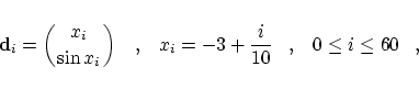
In order to construct a non-uniform B-spline curve containing some maybe unwanted wiggles we proceeded as follows: We started with a planar
cubic B-spline curve ( ) having the 61 control points ) having the 61 control points
and being defined over an equidistant knot vector with  -fold knots at the
two ends. Then 57 inner control points were disturbed with help of random
numbers whereby the maximal allowed disturbance of each control point was 0.02
absolute. Next, we removed 26 interior knots using an automatic algorithm
recently developed by the two authors (Eck and Hadenfeld, 1994a) in order to
end up with a non-uniform disturbed B-spline. Here the bound of the maximal
allowed knot removal error was preselected to 0.01 whereby -fold knots at the
two ends. Then 57 inner control points were disturbed with help of random
numbers whereby the maximal allowed disturbance of each control point was 0.02
absolute. Next, we removed 26 interior knots using an automatic algorithm
recently developed by the two authors (Eck and Hadenfeld, 1994a) in order to
end up with a non-uniform disturbed B-spline. Here the bound of the maximal
allowed knot removal error was preselected to 0.01 whereby  continuity
was preserved at both end points. The final curve is shown in
Fig. 2, and only for completeness we also list the underlying
knot vector: continuity
was preserved at both end points. The final curve is shown in
Fig. 2, and only for completeness we also list the underlying
knot vector:
Figure 2: Given B-spline curve of example 1.
 |
Following criterion (C2), the curvature of the curve is drawn as porcupines to make all the wiggles and unfair regions visible. We have chosen these porcupines,
because we only want to illustrate the shape of the curvature here. The porcupines
are scaled large enough and equal in every picture. Further in the curves shown in
this section all knots are marked.
For the actual fairing of that curve
we selected the two open parameters to be  _ _ = 34
and = 34
and  what exactly is identical to the summed amount of the
disturbance and the knot removal error. The fairing results (each obtained in
0.09 CPU-seconds after 272 control point changes) are as follows: In
Fig. 3a the fairness criterion what exactly is identical to the summed amount of the
disturbance and the knot removal error. The fairing results (each obtained in
0.09 CPU-seconds after 272 control point changes) are as follows: In
Fig. 3a the fairness criterion  is applied whereas in
Fig. 3b criterion is applied whereas in
Fig. 3b criterion  is used. is used.
Figure 3: B-spline curve faired with criterion (a) and (b).
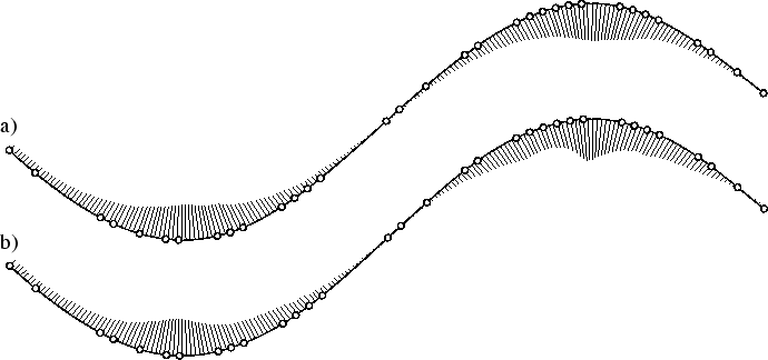 |
It is obvious that both curves are much smoother than the disturbed curve
in Fig. 2 and at least the porcupines in Fig. 3a
are in a rather good shape now. The curve in Fig. 3b is not
totally convincing since the porcupines are more uneven or wavy. Moreover
an unexpected inflection point is appearing at the right end point.
However, such end point inflections can always happen here because we let the two
control points at each boundary unchanged during the fairing process. So in
Fig. 3b this inflection point would vanish if we only would fix
one control point at each boundary.
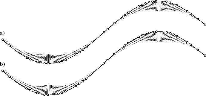
Next we look at the fairing results if the number of ranking list loops is increased
considerably. So for _ = 1000 and again we
obtain the results illustrated in Fig. 4 (each obtained in
0.37 CPU-seconds after 15500 total control point changes). Now we realize that both
curves are in really good shape according to the porcupines. Moreover, the result
from is even better than the one from . Also the end point inflection
has vanished.
Figure 4: B-spline curve faired with criterion (a) and (b).
 |
This observation however seems to be true in general. In order to get satisfying
results using criterion one has to execute the algorithm a large number
of times. But then the results may (not in every case, as we will see later)
even be better than the one obtained with . That means that the velocity of
convergence is much smaller in the case of . This indolent behaviour is not
advantageous for the CPU-time behaviour of our algorithm. However, to be able to
compare the two criteria we will choose large numbers for _ also
in the remaining examples.
In (17) and (18), it is obvious that not only the control
points but also the knot vector with respect to the quality of the
parameterization is important for the fairing results. To illustrate this effect
we took the control points of example 1 and changed manually 9 entries of the knot
vector to
in order to create the second example. The resulting curve is shown in
Fig. 5 where the bad knot distribution on the curve now causes
additional wiggles. The changed knots are displayed as filled dots.
Please note that we could not introduce double knots here
because of the assumption of at least  -fold knots, made before. -fold knots, made before.
Figure 5: Given B-spline of example 2.
 |
Then this new B-spline curve is faired with _ = 1000 and . The result is again obtained in 0.37 CPU-seconds after
15500 iterations (see Fig. 6). Here, it is obvious that the
faired curves are not in such a good shape as before what clearly is an effect
of the unfavourable parameterization of the underlying curve.
Figure 6: B-spline curve faired with criterion (a)
and (b).
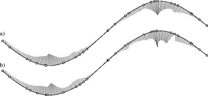 |
Now, the first curve (derived from ) is obviously better. Here all
porcupines point at least into the expected direction. That is even not the
case for the faired curve with which contains two (nearly invisible)
inflection points in the interior.
So, our somewhat subjective conclusion, obtained from many practical tests,
is that the energy integral has in general less problems with these kind
of parameterizations. Altogether, the resulting curves appear more stiff or stable in such situations at least for cubic splines which we mainly
considered.
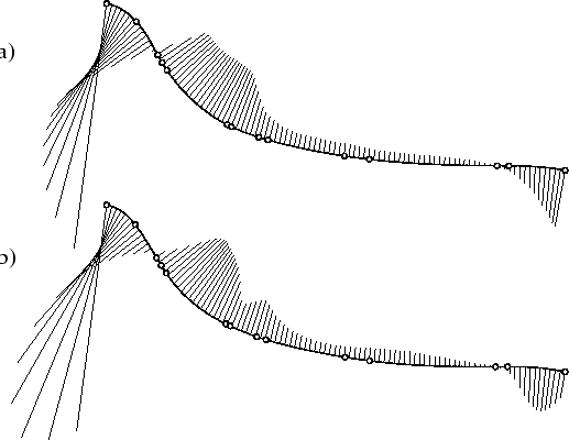
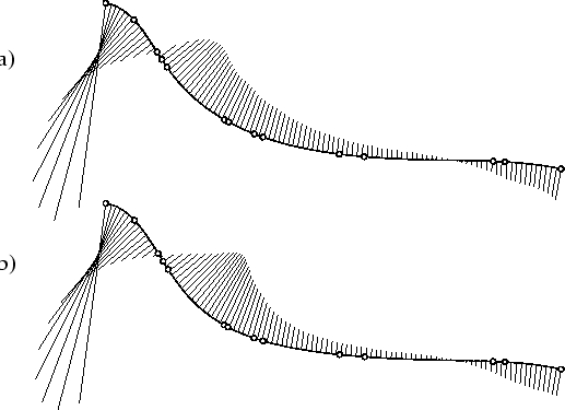
The third example presented here is a boundary curve of a Bézier spline surface
named Surf B and originating from the car body industry; see (Eck and
Hadenfeld, 1994b) for details. This Bézier spline curve of degree  has at first
been converted to a B-spline curve with simple interior knots
(see Fig. 7a).
Then 14 inner control points are additionally disturbed with help of random numbers
(see Fig. 7b) whereby the maximal disturbance at each
control point is at least 3.0 absolute. The disturbance in this case is larger
than in the first two examples because the distance from the first to the
last control point is nearly 367 units. has at first
been converted to a B-spline curve with simple interior knots
(see Fig. 7a).
Then 14 inner control points are additionally disturbed with help of random numbers
(see Fig. 7b) whereby the maximal disturbance at each
control point is at least 3.0 absolute. The disturbance in this case is larger
than in the first two examples because the distance from the first to the
last control point is nearly 367 units.
Figure 7: Given B-spline curve (a) and with a maximal
disturbance of 3.0 (b).
 |
Using the fairness criteria and with  and _ = 1000, the fairing results (obtained in 0.44 CPU-seconds
after 7000 iterations) can be seen in Fig. 8.
Here, both results are nearly perfect meaning that the curvature
distribution is obviously
even better than the one of the original curve in Fig. 7a. and _ = 1000, the fairing results (obtained in 0.44 CPU-seconds
after 7000 iterations) can be seen in Fig. 8.
Here, both results are nearly perfect meaning that the curvature
distribution is obviously
even better than the one of the original curve in Fig. 7a.
Figure 8: B-spline curve faired with criterion (a)
and (b).
 |
Altogether we can recommend the usage of the fairing criterion because
it is not so susceptible for bad parameterizations and moreover a suitable result
is obtained after fewer iteration steps (meaning fewer CPU-time). However, it
is always worth to try also the criterion if (nearly) real-time behaviour is
not required. |