DR. JAN HADENFELD
		A simple extension of the algorithm We have seen in the last part that the two cases of minimization with respect to $E_2$ and to $E_3$ can be interpreted as two extreme cases. This behaviour is also documented in (Meier, 1987) where the variation of the curvature is considered. Therefore, for practical applications Meier proposed the following mixture of both energy integrals $$M = \alpha \cdot E_2 + \beta \cdot E_3 \;\;\;,\;\;\; \alpha,\beta \ge 0\;,\;\alpha + \beta = 1$$ (29) which is claimed to be technically optimal. Here, the values $\alpha$ and $\beta$ must be preselected by the user. Now, in our algorithms we can also minimize $M$ with respect to $\widetilde{\mbox{\bf d}}_r$ in every iteration step. Then it follows by simple calculations that the new location of $\widetilde{\mbox{\bf d}}_r$ is computed by $$\widetilde{\mbox{\bf d}}_r = \bar{\alpha} \cdot \widetilde{\... ...mbox{\bf d}}_r''' \;\;\;,\;\;\; \bar{\alpha} + \bar{\beta} = 1$$ (30) whereby $\widetilde{\mbox{\bf d}}_r''$ resp. $\widetilde{\mbox{\bf d}}_r'''$ represents the solution with respect of $E_2$ resp. $E_3$. Further the weight factors $\bar{\alpha}$, for instance, is given by $$\bar{\alpha} = \frac {\displaystyle \alpha \cdot \int_a^b \l... 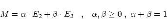...a \cdot \int_a^b \left( N_{r,k}^{(3)} \right)^2 \; dt} \;\;\;.$$ (31) Now, from (30) we further notice that every point of the connecting line of $\widetilde{\mbox{\bf d}}_r''$ and $\widetilde{\mbox{\bf d}}_r'''$ can be interpreted uniquely as a solution of (29) for certain fixed values of $\alpha$ and $\beta$. 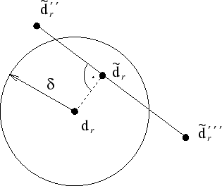This observation can be used to keep the changing of the curve as small as possible in every iteration step of our fairing algorithms. 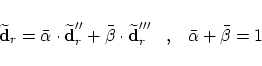Doing so, we define $\widetilde{\mbox{\bf d}}_r$ to be that point on the connecting line which is as close as possible to $\mbox{\bf d}_r$ whereby $\widetilde{\mbox{\bf d}}_r$ always has to lie between $\widetilde{\mbox{\bf d}}_r''$ and $\widetilde{\mbox{\bf d}}_r'''$. This idea is illustrated in Fig. 9, for the planar case. Figure 9: The idea of the mixed energy method. 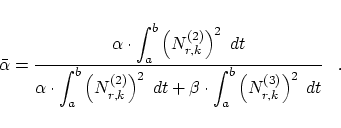So, obviously a different value of $\alpha$ (resp. $\beta$) is chosen in every step. Therefore, we have found an automatic determination of these values which are usually preselected. But because the value $\alpha$ is changed in every iteration step, the convergence of the algorithm is not ensured. Nevertheless, we obtained good results with this procedure. Figure 10: Automatic fairing with the mixed energy method. 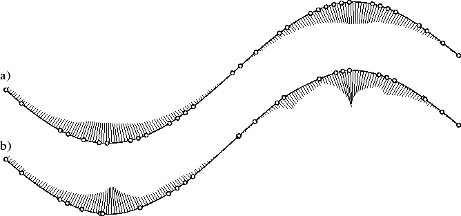In Fig. 10 the fairing results of the mixed energy method for the curves as given in Fig. 2 and Fig. 5 are demonstrated. We used the same B-spline curves to be able to compare the results.