DR. JAN HADENFELD
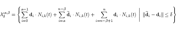
		General discussion The algorithm described thoroughly in the previous section automatically fairs a B-spline curve $\mbox{\bf x}$ of general order $k$ as given in (2). In more detail, our method computes an approximative local solution of the following problem for preset values $\;\delta \geq 0\;$ and $\;\alpha , \beta > 0 \;$: Find a curve $\widetilde{\mbox{\bf x}}$, contained in the set $${\cal X}_{\delta}^{\alpha,\beta} = \left \{ \sum_{i=0}^{\alp... ...e{\mbox{\bf d}}_i - \mbox{\bf d}_i \Vert \leq \delta \right \}$$ (32) of B-splines in the $\delta$-neighborhood of $\mbox{{\bf x}}$ with agreeing boundary values, which satisfies $$\int_{t_{k-1}}^{t_{n+1}} \left(\widetilde{\mbox{\bf x}}^{(l)... ... \;\;\; \mbox{\bf y} \in {\cal X}_{\delta}^{\alpha,\beta} \; .$$ (33) Now, trying to find an (approximative) solution $\widetilde{\mbox{\bf x}}$ with help of well-known optimization methods for nonlinear inequality-constrained problems, as described e.g. in (Gill et al., 1981), is certainly very time consuming for large $n$ since such algorithms require iteratively the solution of a large linear system. Hence the need of any kind of simplification is obvious. 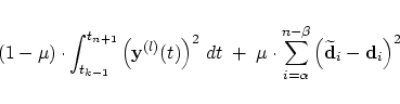One possibility can be found in the already mentioned paper of Kallay (1993) where the quadratic functional $$(1 - \mu) \cdot \int_{t_{k-1}}^{t_{n+1}} \left(\mbox{\bf y}^... ...} \left( \widetilde{\mbox{\bf d}}_i - \mbox{\bf d}_i \right)^2$$ (34) with any preset value $0 \leq \mu \leq 1$ is minimized for $\mbox{\bf y} \in {\cal X}_{\infty}^{\alpha,\beta}$ (meaning the set of all B-splines with same boundary values as $\mbox{\bf x}$). Here, the solution is found by inverting a linear system of magnitude $(n-\alpha -\beta+1) \times (n-\alpha -\beta+1)$. Nevertheless, two disadvantages occur in this method. At first, for $\, \mu \neq 0 \,$ a different functional is minimized as originally stated so that the resulting smoothing effect is not optimal. Secondly, the restrictions (23) are not necessarily fulfilled for the preset value $\mu$ so that one or more iterations with raised values of $\mu$ might be necessary. 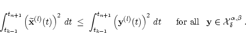So, in contrast to Kallay's method the idea used in the present paper seems to be more practical because the right functional is minimized in every step and the restrictions (23) are always hold. Further, the implementation is much simpler because no linear equation solver is used. However, our method only produces a local approximative solution to the above addressed problem. Nevertheless the (weak) convergence of the iterative process is at least guaranteed since the always positive value of the energy is lowered in every step, producing a bounded decreasing sequence. Moreover, any kind of statement about convergence of the algorithm to a global solution can be given only in the unrestricted case, meaning $\, \delta = \infty\,$, with $\, \alpha , \beta \geq l\,$ and $\,k \geq 2 l\,$. 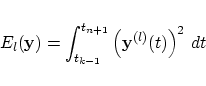In that case the problem of minimizing the positive definite quadratic functional $$E_l(\mbox{\bf y}) = \int_{t_{k-1}}^{t_{n+1}} \left(\mbox{\bf y}^{(l)}(t)\right)^2 \, dt$$ (35) for $\mbox{\bf y} \in {\cal X}_{\infty}^{\alpha,\beta}$ is reduced to the computation of the unique solution of a linear system of magnitude $(n-\alpha -\beta+1) \times (n-\alpha -\beta+1)$ as mentioned above. Note that the resulting solution only depends on the boundary values of the given curve $\mbox{\bf x}$. Now, it is easy to see that our local fairing algorithm tends in the limit to the same global solution. The reason for this behaviour is the possible comparison of our local fairing step to the usual Gauss-Seidel iteration for linear systems (Golub and van Loan, 1989). There in each single step also only one of the unknowns is altered in order to satisfy one equation of the entire linear system exactly. Then in the next step the most recently available information is used to alter the next variable. However, it follows from (25) that the limit of our algorithm is characterized by $\, z_r = 0 \,$ for $\, r=\alpha, \ldots , n-\beta \,$ since otherwise the value of the energy could be lowered by changing some further points. Hence we can deduce from (27) that $\, \bar{\mbox{\bf d}}_r = \widetilde{\mbox{\bf d}}_r \,$ for $\, r=\alpha, \ldots , n-\beta \,$, meaning that every equation of the underlying linear system is satisfied. Thus the obtained limit curve is identical to the global unique solution. For instance in the cubic case ($k=4$) the minimization of $E_2(\mbox{\bf y})$ with $\mbox{\bf y} \in {\cal X}_\infty^{2,2}$ gives for general knot vectors $T$ that cubic Hermite polynomial as limiting curve which interpolates the boundary values $\mbox{\bf x}(t_{k-1})$, $\mbox{\bf x}'(t_{k-1})$, $\mbox{\bf x}(t_{n+1})$ and $\mbox{\bf x}'(t_{n+1})$. Finally, we mention that our algorithm converges for the same reasons also to a global minimum if the restrictions $\, \alpha , \beta \geq l\,$ and $\,k \geq 2 l\,$ are not satisfied. Here, it is much more difficult to predict the limit curve in cases where the global problem has no unique solution since then the limit curve mainly depends on the order the control points are changed.