DR. JAN HADENFELD
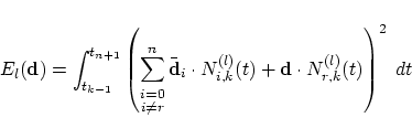
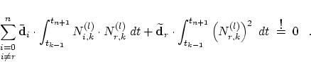
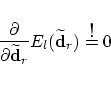
		Computation of the new control point Writing down the energy integral (12) in more detail for a general point $\mbox{\bf d} \in \ifmmode{I\hskip -3pt R} \else{\hbox{$I\hskip -3pt R$}}\fi ^s$ we get $$E_l(\mbox{\bf d}) = \int_{t_{k-1}}^{t_{n+1}} \left( \sum_{\s... ...{(l)}(t) + \mbox{\bf d} \cdot N_{r,k}^{(l)}(t) \right)^2 \; dt$$ (14) representing a quadratic function in $\mbox{\bf d}$. However, we note as an interesting fact that in the planar case ($s=2$) the real contour lines of $E_l(\mbox{\bf d})$ are concentric circles with the unique minimum $\widetilde{\mbox{\bf d}}_r$ as common centre. This observation (valid in a similar way in higher dimensions) will be used later on to control the deviation $\delta$. The unique minimum $\widetilde{\mbox{\bf d}}_r$ itself is determined by $${\partial \over \partial \widetilde{\mbox{\bf d}}_r} E_l(\widetilde{\mbox{\bf d}}_r) \buildrel \mbox{\large !} \over = 0$$ (15) and inserting (14) we obtain from (15) $$\sum_{\stackrel{\scriptstyle i=0}{\scriptstyle i \ne r}}^n \... ...ight)^2 \; dt \; \buildrel \mbox{\large !} \over = \;0 \;\;\;.$$ (16) This single (vector valued) normal equation can be solved simply. If we additionally take advantage of $N_{r,k}^{(l)} \equiv 0$ for $t \notin [t_r,t_{r+k}]$ the solution is $$\widetilde{\mbox{\bf d}}_r = \sum_{\stackrel{\scriptstyle i=... ...criptstyle i \ne r}}^{i_1} \gamma_i \cdot \bar{\mbox{\bf d}}_i$$ (17) with weighting factors $\gamma_i$ of the form $$\gamma_i = - \frac {\displaystyle \int_a^b N_{i,k}^{(l)} \cd... ...aystyle \int_a^b \left( N_{r,k}^{(l)} \right)^2 \; dt} \;\;\;.$$ (18) Here, some further abbreviations have been already incorporated which are necessary to restrict the integration to the curve interval $[t_{k-1},t_{n+1}]$ only: $$a = \max \{ t_r,t_{k-1}\} \;\;\mbox{and}\;\; b = \min \{ t_{r+k},t_{n+1} \}\;\;\;,$$ (19) $$i_0 = \max \{ 0,r-k+1 \} \;\;\mbox{and}\;\; i_1 = \min \{ r+k-1,n \} \;\;\;.$$ (20) Moreover, we notice that $\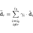widetilde{\mbox{\bf d}}_r$ is computed in (17) by an affine combination of the neighbouring control points $\{ \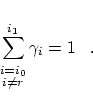bar{\mbox{\bf d}}_i \}$ because we can deduce the following identity from (18) $$\sum_{\stackrel{\scriptstyle i=i_0}{\scriptstyle i \ne r}}^{i_1} \gamma_i = 1 \;\;\; .$$ (21) 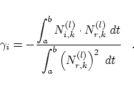However, it seems to be a disadvantage that no closed explicit formula depending only on the actual knot vector $T$ is known for the weights $\gamma_i$ in (18). Nevertheless, the weights $\gamma_i$ can be computed exactly in a finite number of operations since we are here dealing with piecewise polynomial basis functions. For example, we can use a numerical integration method like Gauss quadrature on each interval which works exactly for polynomials of degree $2(k-l-1)$ in order to calculate the appearing integrals in (18). For more details on integrating products of B-splines we refer to (Vermeulen et al., 1992). 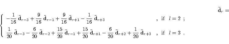Again, in the very special case of an equidistant knot vector $T$ and cubic B-spline curves we can state the formula (17) explicitly: $$\widetilde{\mbox{\bf d}}_r = \left\{ \begin{array}{ll}\disp... ...d}}_{r+3} & ,\;\; \mbox{if} \;\;\; l=3\;\;. \end{array}\right.$$ (22) Here, it is especially remarkable for $l=2$ in (22) that the two control points $\bar{\mbox{\bf d}}_{r-2}$ and $\bar{\mbox{\bf d}}_{r+2}$ do not appear what is of course not valid for general knot vectors $T$. Nevertheless, similar interpretations as possible for formula (8) can be also derived in the present cases: $\bullet$ consider the interpolating cubic polynomial $\mbox{\bf c}(t)$ satisfying $\mbox{\bf c}(-3)=\bar{\mbox{\bf d}}_{r-3}$, $\mbox{\bf c}(-1)=\bar{\mbox{\bf d}}_{r-1}$, $\mbox{\bf c}(1)=\bar{\mbox{\bf d}}_{r+1}$, $\mbox{\bf c}(3)=\bar{\mbox{\bf d}}_{r+3}$, then, for $l=2$, (22) is equivalent to $\widetilde{\mbox{\bf d}}_r=\mbox{\bf c}(0)$; $\bullet$ consider the interpolating quintic polynomial $\mbox{\bf q}(t)$ satisfying $\mbox{\bf q}(-3)=\bar{\mbox{\bf d}}_{r-3}$, $\mbox{\bf q}(-2)=\bar{\mbox{\bf d}}_{r-2}$, $\mbox{\bf q}(-1)=\bar{\mbox{\bf d}}_{r-1}$, $\mbox{\bf q}(1)=\bar{\mbox{\bf d}}_{r+1}$, $\mbox{\bf q}(2)=\bar{\mbox{\bf d}}_{r+2}$, $\mbox{\bf q}(3)=\bar{\mbox{\bf d}}_{r+3}$, then, for $l=3$, [4] (22) is equivalent to $\widetilde{\mbox{\bf d}}_r=\mbox{\bf q}(0)$.