DR. JAN HADENFELD
		Knot removal - knot reinsertion fairing As already mentioned above the iterative local fairing method for planar cubic B-spline curves of Farin and Sapidis is based on fairing criterion (C2). In detail they observed the following: if the discontinuity $$z_i = \vert \dot{\kappa}(t_i^-) - \dot{\kappa}(t_i^+) \vert \;\;\;,\;\;\; 4 \le i \le n$$ (3) of the slope of the curvature (now differentiated with respect to the arc length) at the inner knot $t_i$ is small then the spline curve ${\mbox{\bf x}}(t)$ consists of few monotone curvature pieces in the neighbourhood of the knot $t_i$. In addition, they concluded that the sum $$\xi = \sum_{i=4}^{n} z_i$$ (4) of all local criteria $z_i$ is a reasonable measure to control the number of monotone curvature pieces of the entire curve. For the iterative fairing algorithm itself they used the property of cubic splines that, if the curve is three (instead of at most two) times differentiable at a point ${\mbox{\bf x}}(t_j)$ then the discontinuity $z_j$ is zero (assuming that the tangent vector does not vanish at $t_j$). Thus, they considered how to change the curve ${\mbox{\bf x}}$ locally so that the continuity order at a knot $t_j$ is raised by one. This process, of course, can be interpreted as a knot removal step with a subsequently performed knot reinsertion of the knot $t_j$. 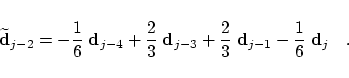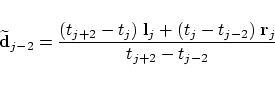Obviously, the simplest way of doing that is to change only one control point namely ${\mbox{\bf d}}_{j-2}$. Then the new location $\widetilde{{\mbox{\bf d}}}_{j-2}$ of this control point is given by $$\widetilde{{\mbox{\bf d}}}_{j-2} = \frac {\displaystyle (t_{... ... 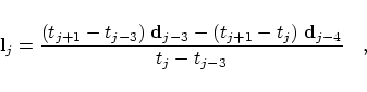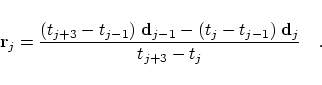t_{j-2}) \; \mbox{\bf r}_j} {\displaystyle t_{j+2} - t_{j-2}}$$ (5) with the two auxiliary points $$\mbox{\bf l}_j = \frac {\displaystyle (t_{j+1} - t_{j-3}) \;... ... \; {\mbox{\bf d}}_{j-4}}{\displaystyle t_j - t_{j-3}} \quad ,$$ (6) $$\mbox{\bf r}_j = \frac {\displaystyle (t_{j+3} - t_{j-1}) \;... ...-1}) \; {\mbox{\bf d}}_j}{\displaystyle t_{j+3} - t_j} \quad .$$ (7) For example, in the special case of an equidistant knot vector $T$ these formulas simplify to $$\widetilde{\mbox{\bf d}}_{j-2} = - \frac{1}{6} \; {\mbox{\bf... ...\mbox{\bf d}}_{j-1} - \frac{1}{6} \; {\mbox{\bf d}}_{j} \quad .$$ (8) Here we note that (8) allows a surprising interpretation: consider the cubic interpolating polynomial $\mbox{\bf c}(t)$ satisfying $\mbox{\bf c}(-4)={\mbox{\bf d}}_{j-4}$, $\mbox{\bf c}(-3)={\mbox{\bf d}}_{j-3}$, $\mbox{\bf c}(-1)={\mbox{\bf d}}_{j-1}$, $\mbox{\bf c}(0)={\mbox{\bf d}}_{j}$, then we simply obtain $\widetilde{\mbox{\bf d}}_{j-2}=\mbox{\bf c}(-2)$. On the other hand, a similar interpretation for general knot vectors could not be found. 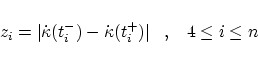We immediately notice that the (faired) curve with $\widetilde{\mbox{\bf d}}_{j-2}$ differs from the original curve only in the interval $]t_{j-2},t_{j+2}[$. Thus this fairing step is local. Several other possibilities to perform this local changing are discussed in (Farin et al., 1987) by varying more than one control point in one local step whereby the changing interval is always increased. Finally, repeating the above local fairing step subsequently at different knots (preferably each time at the knot with the largest value of $z_j$) Farin and Sapidis have found out in several numerical tests that the global criterion $\xi$ from (4) always decreases if the iteration number is only large enough. Altogether, they formulated the following automatic fairing algorithm: Compute $\xi$ and $z_i \; ; \; 4 \le i \le n \;$. Find $z_j = \max \{ z_i \; : \: 4 \le i \le n \} \;$. Compute the new location $\widetilde{\mbox{\bf d}}_{j-2}$ of ${\mbox{\bf d}}_{j-2}$ according to (5) - (7). If a suitable criterion to stop is fulfilled then exit else goto step 1. As possible interruptions in (Sapidis and Farin, 1990) it is suggested either to restrict the number of iterations or to stop if $\xi$ increases resp. if the actual changing of $\xi$ is small enough. Further, a restriction of the new location $\widetilde{\mbox{\bf d}}_{j-2}$ can be built in if a prescribed tolerance of the deviation should be fulfilled. Several examples in (Sapidis and Farin, 1990) illustrate that the fairing algorithm works well in most cases. Nevertheless, the following peculiarities and questions arise: (i) the minimization of $\xi$ is not ensured in every iteration step, (ii) the method is restricted to cubic B-spline curves, (iii) is the local criterion also useful for space curves? (iv) the new location $\widetilde{\mbox{\bf d}}_{j-2}$ only depends on the four neighbouring control points ${\mbox{\bf d}}_{j-4}$, ${\mbox{\bf d}}_{j-3}$, ${\mbox{\bf d}}_{j-1}$, ${\mbox{\bf d}}_j$ although ${\mbox{\bf d}}_{j-5}$ and ${\mbox{\bf d}}_{j+1}$ also influence the interval $]t_{j-2},t_{j+2}[$. All these aspects are evaded in the new iterative fairing method described in the next section.