next up previous
Next: Fairing of B-Spline Surfaces Up: Fairing of B-Spline Curves Previous: Fairing of Rational B-Spline
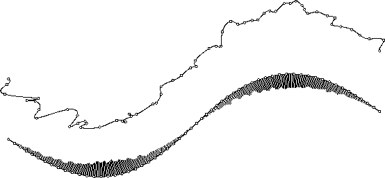
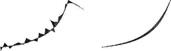
Examples

For the example shown in figure 7 the curve from figure 5 was handled as a rational curve with $w_i = 1$. Then the control points and the weights of the curve were disturbed with the help of random numbers. Because of the numerical quadrature the CPU-time is much larger than in the non-rational case.

Figure: The disturbed rational B-spline curve and the faired one (max_error=$0.82\%$, $0.43$ sec.).
\begin{figure}\centerline{\epsfxsize 130mm \epsfbox{sinus_ori_rat.ps}}\end{figure}

Figure: The disturbed rational B-spline curve and the faired one (max_error=$0.64\%$, $8.523$ sec.).
\begin{figure}
\centerline{\hfill
\epsfxsize 70mm \epsfbox{t_dist.ps} \hfill \epsfxsize 70mm \epsfbox{t_smooth.ps} \hfill}\end{figure}