DR. JAN HADENFELD
| Next: Example Up: Fairing of B-Spline Curves Previous: Examples
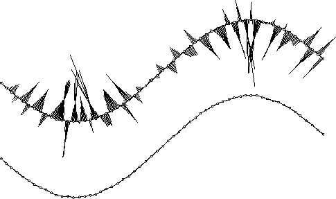
Extension to sets of Bézier- and B-Spline CurvesIf a designer constructs a curve in a way that he splits this curve into a set of Bézier- or B-splines, one possible solution to smooth these curves is to handle each one separately and fix as much as needed control points at the connections to hold the continuity. But by using this method it is not possible to control the whole shape of the curve.A further method is to convert the curves into one B-spline curve. This can easily be done by using a knot-vector with multiple inner knots. If the degrees of the curves are not all the same we have to do a degree elevation to the highest one. By the way, this is also the procedure if you import a VDA-FS file into your CAD system. By fairing this B-spline curve with degree-folded inner knots the result may look like the curve in figure 5.
The shown segments of the curve are smooth (they are nearly lines) whereas the whole curve is not smooth as the continuity of the segments is not optimized. To avoid this, two possible extensions will be described:
The usual way to construct a set of splines is to obtain a continuity at the
connecting points of at least
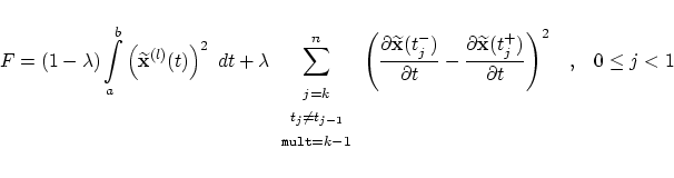
In the cases, the curve is not overall The second extension is to optimize not only the energy functional but also
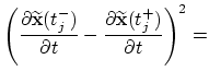
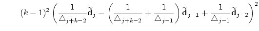
the continuity at the inner knots. By doing so the extended fairness functional
we obtain
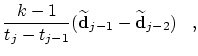
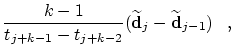
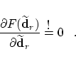
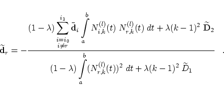
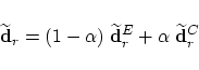
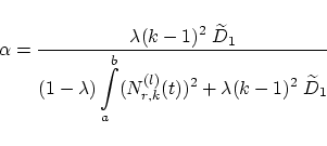
with the abbreviation To find the optimal control point
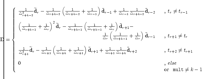
After some calculations and with the following abbreviations
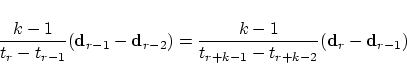
Another spelling for (31) is
In the special case of a cubic B-spline curve with an uniform knot vector,
the new control points are determined by (for 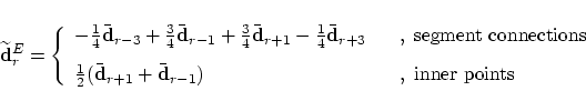 and 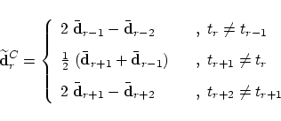 |
|||||||||||||||||||||||||||
![\begin{displaymath}
\bar{\bf d}_i =
\left\{
\begin{array}[c]{ll}
{\bf d}_i & ,...
...f d}_{i+1} & ,\;\;\;r \le i \le n-1\;\;\;.
\end{array}\right.
\end{displaymath}](img75.png)