DR. JAN HADENFELD
| Next: Extension to sets of Up: Fairing of B-Spline Curves Previous: The Algorithm
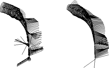
ExamplesThe next given three examples are benchmark curves of the workshop in Lambrecht which have to be faired. In all cases only one control point on each side is fixed and the maximum perpendicular error (max_error) is given in relation to the maximal diagonal. All calculations had been done on a HP 9000/735 workstation. In the first example the curve is a spatial one. To get a better impression
the values of the curvature are not plotted as porcupines but as circles and
the direction of the normals are visualized as lines1. The fairing result in the case of
minimizing the second derivative is not of the same quality as in the case of
the third derivative. The reason could be that by minimizing
the third derivative this integral is the linearization of
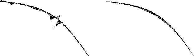
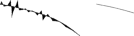
The second and third curves are nearly planar. Only the porcupines here are plotted to visualize the fairness of the curves.
|