DR. JAN HADENFELD
		The New Control Point First of all we introduce the following notations to make a distinction of the different stages of the curve: The given curve which is to be faired: $${\bf x}(t) = \sum_{i=0}^n {\bf d}_i \cdot N_{i,k}(t) \;\;\;,\;\;\;t \in [t_{k-1}, t_{n+1}]\;\;\;.$$ (9) The B-spline curve which has already been faired by a certain number of iterations: $$\bar{\bf x}(t) = \sum_{i=0}^n \bar{\bf d}_i \cdot N_{i,k}(t) \;\;\;,\;\;\;t \in [t_{k-1}, t_{n+1}]\;\;\;.$$ (10) The new curve in the next iteration step: $$\widetilde{\bf x}(t) = \sum_{\stackrel{\scriptstyle i=0}{\sc... ... \cdot N_{r,k}(t) \;\;\;,\;\;\;t \in [t_{k-1}, t_{n+1}]\;\;\;.$$ (11) Here we restrict the index $r$ by $\alpha \le r \le \beta$ to achieve a wanted continuity between the original and the faired B-spline curve. If the curve is also a part of a set of curves and has any continuity with respect to its neigbours it may be wanted to fix the boundaries. 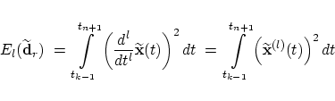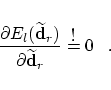Our task now is to find a new location for the control point $\widetilde{\bf d}_r$ in (11) in such a way that the curve $\widetilde{\bf x}(t)$ minimizes the fairness functional. This local minimization problem $$E_l(\widetilde{\bf d}_r) \;=\; \int \limits_{t_{k-1}}^{t_{n+... ...k-1}}^{t_{n+1}} \left( \widetilde{\bf x}^{(l)}(t) \right)^2 dt$$ (12) is a quadratic form in $\widetilde{\bf d}_r$. It has a unique minimum and can be solved explicitly. Here we introduce the value $l$, where $l=2$ or $l=3$ are appropriate choices. Inserting the curve (11) into (12), the unique minimum $\widetilde{\bf d}_r$ is determined by $$\frac{\displaystyle \partial E_l(\widetilde{\bf d}_r)}{\disp... 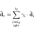...rtial \widetilde{\bf d}_r} \buildrel \hbox{!} \over = 0\;\;\;.$$ (13) This equation can be solved explicitly for the control point $\widetilde{\bf d}_r$ and we obtain $$\widetilde{\bf d}_r = \sum_{\stackrel{\scriptstyle i=i_0}{\scriptstyle i \ne r}}^{i_1} \gamma_i \cdot \bar{\bf d}_i$$ (14) with the weighting factors $\gamma_i$ of the form $$\gamma_i = - \frac {\displaystyle \int_a^b N_{i,k}^{(l)}(t)\... 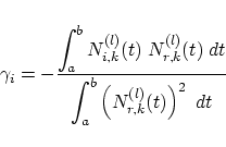...displaystyle \int_a^b \left( N_{r,k}^{(l)}(t) \right)^2 \; dt}$$ (15) and the following abbreviations for the limits of the integrals and the sum: $$\begin{eqnarray*} a = \max \{ t_r,t_{k-1}\} & \;\;\mbox{and}\;\; & b = \min \{ ... ...,r-k+1 \}& \;\;\mbox{and}\;\; & i_1 = \min \{ r+k-1,n \} \;\;\;. 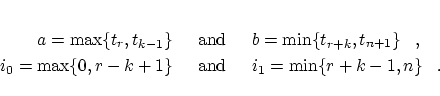\end{eqnarray*}$$ To control the calculation of the integrals we can use the property that the control point $\widetilde{\bf d}_r$ is an affine combination of the neighbouring control points because of $$\sum_{\stackrel{\scriptstyle i=i_0}{\scriptstyle i \ne r}}^{i_1} \gamma_i = 1 \;\;\; .$$ (16) The integrals could be calculated exactly with the help of Gaussian quadrature. Further information can be found in [31].